First things first. To work with any FE model, we need a mesh! In this article I will present how to:

• Build and plot an unstructured mesh.
• Animate a mesh and a node or cell scalar field.

The tools we will use are:

• Gmsh: A FE mesh generator.
• Gmsh.jl: API package to use Gmsh in Julia.
• Paraview: A powerful visualization application.
• WriteVTK.jl: Create Paraview files from Julia.

Build and plot a 2D unstructured mesh.

This mesh_gmsh.jl function allows us to create a simple 2D mesh, showing it with gmsh.fltk.run(), and saving it into a .msh file.

Calling this function with arguments b = 1e-2, h = 1e-2, lc = 1e-3, filename = "mesh_1" will produce a square with side of 1 cm, and a mesh size of 1 mm, the file will be saved as “mesh_1.msh”. Here we see the plot created after calling the function.

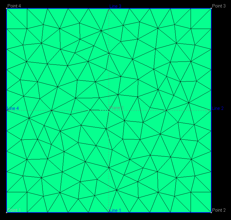
More importantly, the function will return the nodes and elements arrays to begin our FE analysis.

Animate a mesh and a node or cell scalar field

WriteVTK.jl is a great package to work with the powerful Paraview visualization application. Thanks to this package, I am able to run real-time animations produced within my Julia code, since Paraview automatically updates the source file for the animations.

In the WriteVTK.jl GitHub page you will find some useful examples of its uses, but here I will share another one, exporting our mesh with time-varying node coordinates.

The animated_mesh.jl uses the previously created mesh and adds some y-displacements that represent simple harmonic motion. Time-dependent animations are created with the WriteVTK.jl package, and the .vtu independent files and .pvd main animation file are stored in the “paraview” folder (you have to create the empty folder previously!).

If you need to work with structured 2D meshes, here I share a struct_mesh.jl function that I’ve created for simple rectangular geometries. In the next post I will write about 3D meshes.